Five Flowers Image Classification in TPU-Enabled Kaggle Instance

As in Google Colab, a TPU-enabled instance in Kaggle needs to be equipped with a Google Cloud Storage (GCS) bucket because for all but a few simple experimentation like tf.data.Dataset.from_tensor_slices() you need to feed TPUs data swiftly enough to make the most of them. In the post I will show you how to load TFRecords to a Kaggle notebook and walk you through typical deep learning workflow that starts with data preprocessing, data splitting, architecture configuration, model training and model validation, all the way to model prediction.

Some code snippets in the text below are copied from Martin Gorner’s excellent work titled “Five flowers with Keras and Xception on TPU” in Kaggle’s forum. I added further elaboration for my future reference.

Loading TFRecords from Subfolders

Suppose the base folder of our dataset is called five-flowers under /kaggle/input. The file system is organized as follows:

/kaggle$ tree -L 3
.
├── input
│   └── five-flowers
│       ├── LICENSE.txt
│       ├── original-jpegs
│       ├── tfrecords-jpeg-192x192
│       ├── tfrecords-jpeg-224x224
│       ├── tfrecords-jpeg-331x331
│       └── tfrecords-jpeg-512x512
├── lib
│   └── kaggle
│       └── gcp.py
└── working
    └── __notebook_source__.ipynb

Each tfrecords-jpeg* represents an image folder. We want to attach these data to the TPU environment we are assigned.

Identifying subfolders of images”. We import the package kaggle_datasets and evoke its function get_gcs_path function to get the list of subfolders under the folder five-flowers.

import re
import os
import tensorflow as tf
import tensorflow_hub as hub
import numpy as np
from matplotlib import pyplot as plt
print("Tensorflow version " + tf.__version__)
AUTO = tf.data.experimental.AUTOTUNE
from kaggle_datasets import KaggleDatasets

# NEW on TPU in TensorFlow 24: shorter cross-compatible TPU/GPU/multi-GPU/cluster-GPU detection code
try: # detect TPUs
    tpu = tf.distribute.cluster_resolver.TPUClusterResolver.connect() # TPU detection
    strategy = tf.distribute.TPUStrategy(tpu)
except ValueError: # detect GPUs
    strategy = tf.distribute.MirroredStrategy() # for GPU or multi-GPU machines
    #strategy = tf.distribute.get_strategy() # default strategy that works on CPU and single GPU
    #strategy = tf.distribute.experimental.MultiWorkerMirroredStrategy() # for clusters of multi-GPU machines

print("Number of accelerators: ", strategy.num_replicas_in_sync)
data_base_folder = 'five-flowers'

GCS_PATH = KaggleDatasets().get_gcs_path(data_base_folder)
!gsutil ls $GCS_PATH

It’s worthy of noting that if your TPU instance is on Google Colaboratory, the first line of the initialization code should be modified to the following (Li-Pin: statement to be verified):

# tpu = tf.distribute.cluster_resolver.TPUClusterResolver(tpu = 'grpc://' + os.environ['COLAB_TPU_ADDR'])

In the code above we pass the data’s base name string as an argument into function get_gcs_path() and then prepend an exclamation mark to gsutil ls followed by the reference to our base name folder. The command line execution returns the list of subfolders under the root directory of the data as shown below:

#output
gs://kds-f4bb9080456bfec141abba97b98332d712767aa5432a96e8e301af1e/LICENSE.txt
gs://kds-f4bb9080456bfec141abba97b98332d712767aa5432a96e8e301af1e/original-jpegs/
gs://kds-f4bb9080456bfec141abba97b98332d712767aa5432a96e8e301af1e/tfrecords-jpeg-192x192/
gs://kds-f4bb9080456bfec141abba97b98332d712767aa5432a96e8e301af1e/tfrecords-jpeg-224x224/
gs://kds-f4bb9080456bfec141abba97b98332d712767aa5432a96e8e301af1e/tfrecords-jpeg-331x331/
gs://kds-f4bb9080456bfec141abba97b98332d712767aa5432a96e8e301af1e/tfrecords-jpeg-512x512/

Creating a dict mapping to track variants of data. Since the data have five variants in terms of image size, we create a hash table to take note of the difference. This step is necessary because generic deep learning models for computer vision is strict with respect to the dimension of input image size. By creating a hash table to track the dimension of image size in each subfolder, we allow deep learning models to load image inputs with appropriate dimensions.

FLOWERS_DATASETS = { # available image sizes
    192: GCS_PATH + '/tfrecords-jpeg-192x192/*.tfrec',
    224: GCS_PATH + '/tfrecords-jpeg-224x224/*.tfrec',
    331: GCS_PATH + '/tfrecords-jpeg-331x331/*.tfrec',
    512: GCS_PATH + '/tfrecords-jpeg-512x512/*.tfrec'
}
CLASSES = ['daisy', 'dandelion', 'roses', 'sunflowers', 'tulips'] # do not change, maps to the labels in the data (folder names)
BATCH_SIZE = 16 * strategy.num_replicas_in_sync # this is 8 on TPU v3-8, it is 1 on CPU and GPU
EPOCHS = 12 
IMAGE_SIZE = [331, 331] #-- suppose we are intersted in image of dimensions (331, 331). 
assert IMAGE_SIZE[0] == IMAGE_SIZE[1], "only square images are supported"
assert IMAGE_SIZE[0] in FLOWERS_DATASETS, "this image size is not supported"

Counting the number of files from a specific subfolder. We utilize regular expression to formulate the pattern for returning the character set 230 from a given string flowers00-230.tfrec for example.

def count_data_items(filenames):
    # the number of data items is written in the name of the .tfrec files, i.e. flowers00-230.tfrec = 230 data items
    n = [int(re.compile(r"-([0-9]*)\.").search(filename).group(1)) for filename in filenames] 
    return np.sum(n)

gcs_paths_desired = FLOWERS_DATASETS[IMAGE_SIZE[0]] # get the gcs paths that contains images of desired dimensions. 
TRAINING_FILENAMES = tf.io.gfile.glob(gcs_paths_desired) # Returns a list of files that match the given pattern(s).
print("TRAINING IMAGES: ", count_data_items(TRAINING_FILENAMES)) # Answer is 3670

Data Preprocessing

Parsing examples according to custom protocol buffer messages. Create a dictionary which maps keys to tf.train.Feature object types. We can think of each key-value pair corresponding to a single feature of a data point. A data point, example, has to be a scalar string Tensor, a single serialized Example. The function tf.io.parse_single_example returns a dict mapping feature keys to Tensor and SparseTensor values (see the API doc for details)

def read_tfrecord(example):  
    features = {
        "image": tf.io.FixedLenFeature([], tf.string), # tf.string means bytestring
        "class": tf.io.FixedLenFeature([], tf.int64),  # shape [] means scalar
        "one_hot_class": tf.io.VarLenFeature(tf.float32),
    }
    example = tf.io.parse_single_example(example, features) #L: Parses a single Example proto.
    # Data Preprocessing Is Done In This Step.
    image = tf.image.decode_jpeg(example['image'], channels=3) # pixel format uint8 [0,255] range
    class_label = tf.cast(example['class'], tf.int32) # not used
    one_hot_class = tf.sparse.to_dense(example['one_hot_class'])
    one_hot_class = tf.reshape(one_hot_class, [5])
    return image, one_hot_class #--- the output structure is ["image", "one_hot_class"]

Preprocessing, augmentation, and transformation TFRecords. The custom function load_dataset() wraps subfunctions into one: (1) TFRecordDataset(), (2) read_tfrecord(), (3) reshape_images(), and after parsing all the data into tf.dataset object, (4) data_augment(). The last three subfunctions are applied at individual data point level along with the call of dataset.map() function.

def force_image_sizes(dataset, image_size):
    # explicit size needed for TPU
    reshape_images = lambda image, label: (tf.reshape(image, [*image_size, 3]), label)
    dataset = dataset.map(reshape_images, num_parallel_calls=AUTO)
    return dataset

def load_dataset(filenames):
    # Read from TFRecords. For optimal performance, reading from multiple files at once and
    # disregarding data order. Order does not matter since we will be shuffling the data anyway.

    ignore_order = tf.data.Options()
    ignore_order.experimental_deterministic = False

    dataset = tf.data.TFRecordDataset(filenames, num_parallel_reads=AUTO) # automatically interleaves reads from multiple files
    dataset = dataset.with_options(ignore_order) # uses data as soon as it streams in, rather than in its original order
    dataset = dataset.map(read_tfrecord, num_parallel_calls=AUTO) #--- Data Preprocessing
    dataset = force_image_sizes(dataset, IMAGE_SIZE) #--- Forcing the dimension change of images
    return dataset

def data_augment(image, one_hot_class):
    # data augmentation. Thanks to the dataset.prefetch(AUTO) statement in the next function (below),
    # this happens essentially for free on TPU. Data pipeline code is executed on the "CPU" part
    # of the TPU while the TPU itself is computing gradients.
    image = tf.image.random_flip_left_right(image)
    image = tf.image.random_saturation(image, 0, 2)
    return image, one_hot_class 

def get_training_dataset():
    dataset = load_dataset(TRAINING_FILENAMES)
    dataset = dataset.map(data_augment, num_parallel_calls=AUTO) #--- Apply data augmentation
    dataset = dataset.repeat()
    dataset = dataset.shuffle(2048)
    dataset = dataset.batch(BATCH_SIZE)
    dataset = dataset.prefetch(AUTO) # prefetch next batch while training (autotune prefetch buffer size)
    return dataset

Generally, input image data’s dimension has to be consistent with what the pretrained model expects. The original dimension of input images is [331, 331]. In Martin Gornor’s code, he didn’t force the dimension to be changed to [299, 299], a image dimension which his pretrained model Xception needs, at the moment. You will see the required image dimension change later.

Besides, if you call .cache() as commonly adopted in practice for deep learning on GPU, TensorFlow will try to cache the dataset on the TPU VM, not on the GCE VM (e.g. n1-standard-2), which should be able to fit huge dataset by default since TPU VM has way more RAM available than the GCE VM. However, in general you do not want to call that when running on TPUs because Google uses GCSFileSystem which does the caching in the background of TFRecord shards.

The takeaway is that don’t use dataset.cache() on TPU instances.

One more note is regarding the order of batch() and repeat(). If you want to have a clear epoch separation, put batch() before repeat() to avoid duplicated examples shown in the same epoch.

Sample Data Visualization

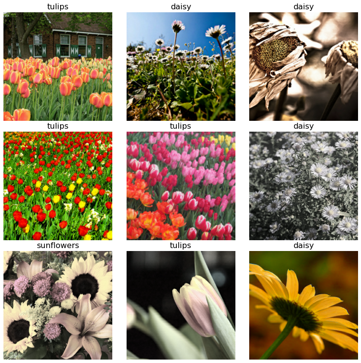
Sampling the resulting tf.dataset object with custom plotting functions.

def dataset_to_numpy_util(dataset, N):
    dataset = dataset.unbatch().batch(N)
    for images, labels in dataset:
        numpy_images = images.numpy()
        numpy_labels = labels.numpy()
        break  
    return numpy_images, numpy_labels

def display_one_flower(image, title, subplot, red=False):
    plt.subplot(subplot)
    plt.axis('off')
    plt.imshow(image)
    plt.title(title, fontsize=16, color='red' if red else 'black')
    return subplot+1

#--- Useless in this tutorial
def title_from_label_and_target(label, correct_label): 
    label = np.argmax(label, axis=-1)  # one-hot to class number
    correct_label = np.argmax(correct_label, axis=-1) #--- compress one-hot vector to class number
    correct = (label == correct_label)
    return "{} [{}{}{}]".format(CLASSES[label], str(correct), ', shoud be ' if not correct else '',
                                CLASSES[correct_label] if not correct else ''), correct

def display_9_images_from_dataset(dataset):
    subplot=331
    plt.figure(figsize=(13,13))
    images, labels = dataset_to_numpy_util(dataset, 9)
    for i, image in enumerate(images):
        title = CLASSES[np.argmax(labels[i], axis=-1)]
        subplot = display_one_flower(image, title, subplot)
        if i >= 8:
            break
    plt.subplots_adjust(wspace=0.1, hspace=0.1)
    plt.show()

training_dataset = get_training_dataset()
display_9_images_from_dataset(training_dataset)

Post-Data-Preprocessing Workflow

Splitting TFRecords into training set and validation set

def get_validation_dataset():
    dataset = load_dataset(VALIDATION_FILENAMES)
    dataset = dataset.batch(BATCH_SIZE)
    dataset = dataset.prefetch(AUTO) # prefetch next batch while training (autotune prefetch buffer size)
    return dataset

gcs_pattern = FLOWERS_DATASETS[IMAGE_SIZE[0]]
validation_split = 0.2
filenames = tf.io.gfile.glob(gcs_pattern)
split = len(filenames) - int(len(filenames) * validation_split)
TRAINING_FILENAMES = filenames[:split]
VALIDATION_FILENAMES = filenames[split:]
TRAIN_STEPS = count_data_items(TRAINING_FILENAMES) // BATCH_SIZE
VALIDATION_STEPS = -(-count_data_items(VALIDATION_FILENAMES) // BATCH_SIZE) # The "-(-//)" trick rounds up instead of down :-)
print("TRAINING IMAGES: ", count_data_items(TRAINING_FILENAMES), ", STEPS PER EPOCH: ", TRAIN_STEPS)
print("VALIDATION IMAGES: ", count_data_items(VALIDATION_FILENAMES))

I would make one more revision on Martin’s work here to shuffle filenames thoroughly before splitting data. This early shuffl gives the dataset more randomness to avoid overfitting in the same spirit as this lecture note by Andrew Ng, rather than leaving the randomization to get_training_dataset() and get_validation_dataset() later on.

Transfer Learning

Note that tensorflow model creation needs to be inside strategy.scope, so the variables can be created on each TPU device. The rest of the code is not needed to be inside the strategy scope.

# Required Keras high level API for distributed training, regardless of whether it is TPUs or multiple GPUs.
with strategy.scope():
    img_adjust_layer = tf.keras.layers.Lambda(lambda data: tf.keras.applications.xception.preprocess_input(tf.cast(data, tf.float32)), input_shape=[*IMAGE_SIZE, 3])
    pretrained_model = tf.keras.applications.Xception(weights='imagenet', include_top=False)

    # alternative: EfficientNetB0
    #img_adjust_layer = tf.keras.layers.Lambda(lambda data: tf.keras.applications.efficientnet.preprocess_input(tf.cast(data, tf.float32)), input_shape=[*IMAGE_SIZE, 3])
    #pretrained_model = tf.keras.applications.EfficientNetB0(include_top=False)
    pretrained_model.trainable = True #L: it's fine because we use a learning rate schedule with ramp up.
    model = tf.keras.Sequential([
        img_adjust_layer,
        pretrained_model,
        tf.keras.layers.GlobalAveragePooling2D(),
        #tf.keras.layers.Flatten(),
        tf.keras.layers.Dense(5, activation='softmax')
    ])
model.compile(
    optimizer='adam',
    loss = 'categorical_crossentropy',
    metrics=['accuracy'],
    # NEW on TPU in TensorFlow 24: sending multiple batches to the TPU at once saves communications
    # overheads and allows the XLA compiler to unroll the loop on TPU and optimize hardware utilization.
    steps_per_execution=8
)

model.summary()

According to the official API doc of the Xception pretrained model, if we discard the top layer of the pretrained model, i.e., include_top = False, we need to specify the input shape. In Martin’s code, he accomplishes this requirement with function xception.preprocess_input() and a Keras Lambda layer. We may choose another pretrained model such as EfficentNetB0 simply by replacing xception with efficientnet in the lines of img_adjust_layer = and pretrained_model =.

A complete process of transfer learning can be broken into two phases: freeze and fine-tuning. In Martin Gornor’s article he adopts a learning rate schedule that considers warm up with respect to the learning rate increment. By doing so, conceptually, the top untrained layer of the model can smoothly learn to work with the pretrained model because of smaller learning rates in the early phase of training.

Besides, the layer next to the last one is set to be a GlobalAveragePooling2D layer rather than a Flatten layer. It’s because the consideration of parameter parsimony. The latter case have more parameters to train and take a little longer to train.

IMPORTANT! As emphasized by Martin Gornor and Francois Chollet (tweet), when running on TPU, you can significantly speed up your model by running multiple steps of gradient descent in a single graph execution (i.e. pass the steps_per_execution argument to Model.compile()). This helps reduce Python overhead and get the device to 100% utilization (which, for a TPU, is huge). If you have implemented a model with a custom train_step method, this feature is automatically available for your custom training loop. This is one of a few advantages of implementing custom training loops via train_step.

As Francois Chollet mentioned (tweet), you don’t need to use steps_per_execution every time you use a TPU (or GPU). It depends on your model. For example, a model like ResNet50 with batch size 256 would already be near full utilization and wouldn’t benefit from it. But a small dense model would have very low utilization, and in this case, you can use this argument to get to 100% utilization without changing your batch size. The speed up you get is inversely proportional to the original utilization – could be 1.5x or 50x. In a related topic, Francois Chollet says “If you’re using Colab and you feel like training your model on GPU is slow, switch to the TPU runtime and tune the steps_per_execution parameter in compile(). Seeing a 5-10x speedup is pretty common.”

Setting the value of steps_per_execution to anything between 2 and steps_per_epoch can help (source: tensorflow api doc).

The takeaway is that steps_per_execution provides you a way to reach full device utilization.

Model training and validation

# Learning rate schedule for TPU, GPU and CPU.
# Using an LR ramp up because fine-tuning a pre-trained model.
# Starting with a high LR would break the pre-trained weights.

LR_START = 0.00001
LR_MAX = 0.00005 * strategy.num_replicas_in_sync
LR_MIN = 0.00001
LR_RAMPUP_EPOCHS = 5
LR_SUSTAIN_EPOCHS = 0
LR_EXP_DECAY = .8

def lrfn(epoch):
    if epoch < LR_RAMPUP_EPOCHS:
        lr = (LR_MAX - LR_START) / LR_RAMPUP_EPOCHS * epoch + LR_START
    elif epoch < LR_RAMPUP_EPOCHS + LR_SUSTAIN_EPOCHS:
        lr = LR_MAX
    else:
        lr = (LR_MAX - LR_MIN) * LR_EXP_DECAY**(epoch - LR_RAMPUP_EPOCHS - LR_SUSTAIN_EPOCHS) + LR_MIN
    return lr
    
lr_callback = tf.keras.callbacks.LearningRateScheduler(lrfn, verbose=True)

rng = [i for i in range(EPOCHS)]
y = [lrfn(x) for x in rng]
plt.plot(rng, y)
print("Learning rate schedule: {:.3g} to {:.3g} to {:.3g}".format(y[0], max(y), y[-1]))

history = model.fit(
    get_training_dataset(), 
    steps_per_epoch=TRAIN_STEPS, 
    epochs=EPOCHS,
    validation_data=get_validation_dataset(), 
    validation_steps=VALIDATION_STEPS,
    callbacks=[lr_callback]
)
final_accuracy = history.history["val_accuracy"][-5:]
print("FINAL ACCURACY MEAN OF LAST FIVE EPOCHS: ", np.mean(final_accuracy))

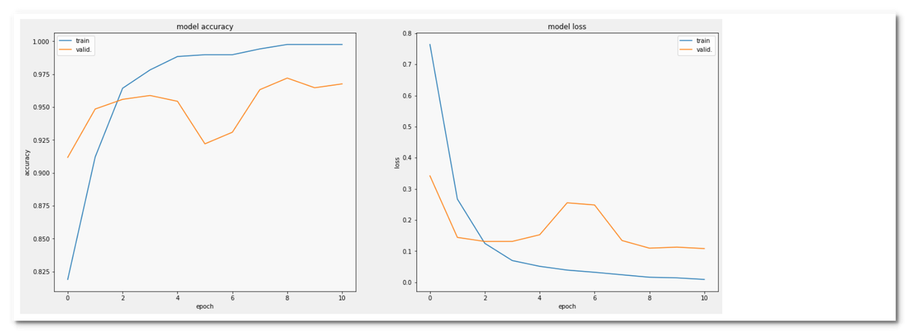
Plotting learning curves

def display_training_curves(training, validation, title, subplot):
    if subplot%10==1: # set up the subplots on the first call
        plt.subplots(figsize=(10,10), facecolor='#F0F0F0')
        #plt.tight_layout()
    ax = plt.subplot(subplot)
    ax.set_facecolor('#F8F8F8')
    ax.plot(training)
    ax.plot(validation)
    ax.set_title('model '+ title)
    ax.set_ylabel(title)
    ax.set_xlabel('epoch')
    ax.legend(['train', 'valid.'])

display_training_curves(history.history['accuracy'][1:], history.history['val_accuracy'][1:], 'accuracy', 121)
display_training_curves(history.history['loss'][1:], history.history['val_loss'][1:], 'loss', 122)

Prediction

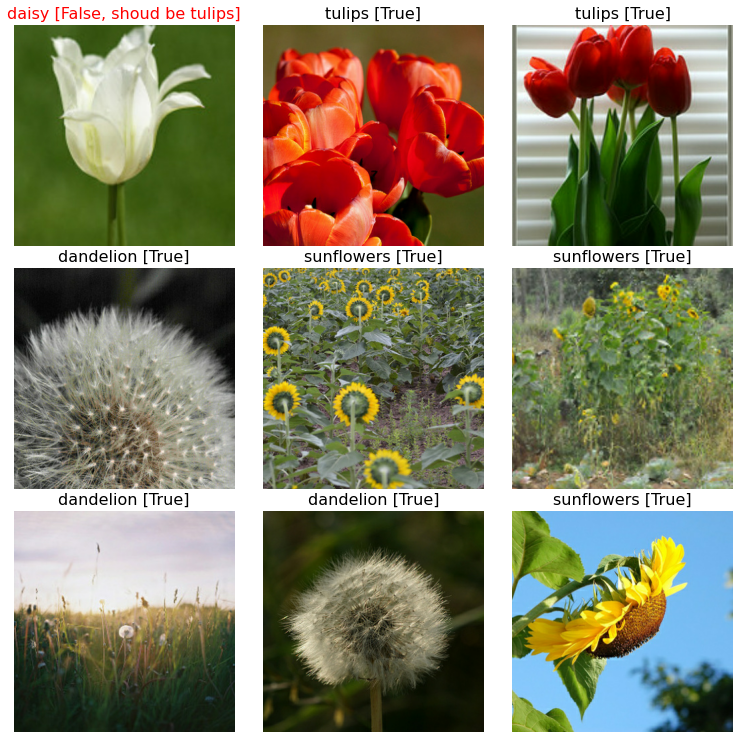
def display_9_images_with_predictions(images, predictions, labels):
    subplot=331
    plt.figure(figsize=(13,13))
    for i, image in enumerate(images):
        title, correct = title_from_label_and_target(predictions[i], labels[i])
        subplot = display_one_flower(image, title, subplot, not correct)
        if i >= 8:
            break
    #plt.tight_layout()
    plt.subplots_adjust(wspace=0.1, hspace=0.1)
    plt.show()

# a couple of images to test predictions too
some_flowers, some_labels = dataset_to_numpy_util(get_validation_dataset(), 160)

# randomize the input so that you can execute multiple times to change results
permutation = np.random.permutation(8*20)
some_flowers, some_labels = (some_flowers[permutation], some_labels[permutation])

predictions = model.predict(some_flowers, batch_size=16)
evaluations = model.evaluate(some_flowers, some_labels, batch_size=16)
  
print(np.array(CLASSES)[np.argmax(predictions, axis=-1)].tolist())
print('[val_loss, val_acc]', evaluations)

display_9_images_with_predictions(some_flowers, predictions, some_labels)

Save the trained model to local disk

A Keras model consists of multiple components:

1. The architecture that specifies what layers it contain and how they’re connected.
2. A set of weight values.
3. An optimizer defined in model.compile().
4. A set of losses and metrics defined in model.compile().

The Keras API makes it possible to save all of these pieces to disk at once in the TensorFlow SavedModel TF format (a SavedModel protocol buffers file; default in TensorFlow 2.x) or in the older Keras H5 (HDF5) format (default in TensorFlow 1.x).

However, the TF format has not worked with TPUs yet (as of February, 2021), as mentioned by Martin Gorner below:

save_locally = tf.saved_model.SaveOptions(experimental_io_device='/job:localhost')
model.save('./model', options=save_locally) # saving in Tensorflow's "saved model" format

Since TensorFlow 2.4 has not supported the feature of saving in TF format, should we pass save_format='h5' or a filename with the extension .h5? It seems not necessary to do either simply based on Martin Gornor’s code. I guess it’s probably because TensorFlow would check if it’s a TPU runtime and switch to the H5 format accordingly.

IMPORTANT! Compared to the SavedModel format, saving a model in the H5 file faces a limitation: external losses and metrics added via model.add_loss() and model.add_metric() are not saved. When loading a model with such a losses and metrics configuration, you need to add them back yourself after loading the model. One exception is that if custom made losses or metrics were created inside layers via self.add_loss() and self.add_metric(), the limitation doesn’t apply.

Reload the trained model locally

# New in Tensorflow 2.4: models can be reloaded locally to TPUs in Tensorflow's SavedModel format
with strategy.scope():
    # TPUs need this extra setting to load from local disk, otherwise, they can only load models from GCS (Google Cloud Storage).
    # The setting instructs Tensorflow do the model loading on the local VM, not the TPU. Tensorflow can then still
    # instantiate the model on the TPU if the loading call is placed in a TPUStrategy scope. This setting does nothing on GPUs.
    load_locally = tf.saved_model.LoadOptions(experimental_io_device='/job:localhost')
    model = tf.keras.models.load_model('./model', options=load_locally) # loading in Tensorflow's "saved model" format

predictions = model.predict(tf.cast(some_flowers, tf.float32), batch_size=16)
evaluations = model.evaluate(tf.cast(some_flowers, tf.float32), some_labels, batch_size=16)
print(np.array(CLASSES)[np.argmax(predictions, axis=-1)].tolist())
print('[val_loss, val_acc]', evaluations)
display_9_images_with_predictions(some_flowers, predictions, some_labels)

References

[1]	Five flowers with Keras and Xception on TPU by Martin Gorner
[2]	Use TPUs, Tensorflow API doc
[3]	Where is data cached when using a Cloud TPU?, StackOverflow
[4]	What is the difference between .pb SavedModel and .tf SavedModel?, StackOverflow
[5]	Save and load Keras models, TensorFlow API doc

Appendix

I. Excerption

For most use-cases, it is recommended to convert your data into TFRecord format and use a tf.data.TFRecordDataset to read it. See TFRecord and tf.Example tutorial for details on how to do this. This, however, is not a hard requirement and you can use other dataset readers (FixedLengthRecordDataset or TextLineDataset) if you prefer.

Source: “Use TPUs” by TensorFlow

II. More Experiments on TPUs

The following two examples comes from the Keras API doc. I revise the original code by enabling the code to run on TPUs.

Saving and loading a regression model example

import tensorflow as tf
def get_model():
    # Create a simple model.
    inputs = tf.keras.Input(shape=(32,))
    outputs = tf.keras.layers.Dense(1)(inputs)
    model = tf.keras.Model(inputs, outputs)
    model.compile(optimizer="adam", loss="mean_squared_error")
    return model

model = get_model()

# Train the model.
test_input = np.random.random((128, 32))
test_target = np.random.random((128, 1))
model.fit(test_input, test_target)

# Calling `save('my_model')` creates a SavedModel folder `my_model`.
save_locally = tf.saved_model.SaveOptions(experimental_io_device='/job:localhost')
model.save('./my_model', options=save_locally)
# It can be used to reconstruct the model identically.
with strategy.scope():
    load_locally = tf.saved_model.LoadOptions(experimental_io_device='/job:localhost')
    reconstructed_model = tf.keras.models.load_model('./my_model', options=load_locally) # loading in Tensorflow's "saved model" format

reconstructed_model.fit(test_input, test_target)

Reference: Keras API doc

Transfer learning example

inputs = keras.Input(shape=(784,), name="digits")
x = keras.layers.Dense(64, activation="relu", name="dense_1")(inputs)
x = keras.layers.Dense(64, activation="relu", name="dense_2")(x)
outputs = keras.layers.Dense(10, name="predictions")(x)
functional_model = keras.Model(inputs=inputs, outputs=outputs, name="3_layer_mlp")

# Extract a portion of the functional model defined in the Setup section.
# The following lines produce a new model that excludes the final output
# layer of the functional model.
pretrained = keras.Model(
    functional_model.inputs, functional_model.layers[-1].input, name="pretrained_model"
)
# Randomly assign "trained" weights.
for w in pretrained.weights:
    w.assign(tf.random.normal(w.shape))
save_locally = tf.saved_model.SaveOptions(experimental_io_device='/job:localhost')
# model.save('./my_model', options=save_locally)
pretrained.save_weights("pretrained_ckpt", options=save_locally)
pretrained.summary()

# Assume this is a separate program where only 'pretrained_ckpt' exists.
# Create a new functional model with a different output dimension.
inputs = keras.Input(shape=(784,), name="digits")
x = keras.layers.Dense(64, activation="relu", name="dense_1")(inputs)
x = keras.layers.Dense(64, activation="relu", name="dense_2")(x)
outputs = keras.layers.Dense(5, name="predictions")(x)
model = keras.Model(inputs=inputs, outputs=outputs, name="new_model")

# Load the weights from pretrained_ckpt into model.
with strategy.scope():
    load_locally = tf.saved_model.LoadOptions(experimental_io_device='/job:localhost')
    model.load_weights("pretrained_ckpt", options=load_locally) # loading in Tensorflow's "saved model" format

# Check that all of the pretrained weights have been loaded.
for a, b in zip(pretrained.weights, model.weights):
    np.testing.assert_allclose(a.numpy(), b.numpy())

print("\n", "-" * 50)
model.summary()

Reference: Keras API doc